Coverage Overlays
See where each terrain or basemap source actually has data, before switching to it
Source Info
Source Info is the Tools-group section that answers "what am I actually looking at?" for whatever is loaded right now. For each active terrain source and basemap it shows:
- the dataset's name, provider and licence, with attribution text ready to copy;
- its resolution — a declared native grid where the dataset states one, otherwise the ground size of one pixel at its maximum zoom at the current latitude (
z19 ≈ 30 cm/px), which is the only honest figure a tile service can give; - the endpoint actually being requested, and a link to the dataset's own page;
- for COGs, links to open the same file in an external viewer (source.coop, GeoLibre);
- and the coverage picker described below.
Sources that arrived from a catalog keep their provenance: an Editor Layer Index layer carries its index entry and licence, a STAC item carries its collection.
It is also where a source found under the cursor can be switched into view A in one click — the hover list below sorts what covers a point by increasing ground sample distance, so the sharpest dataset available there is first.
Coverage overlays
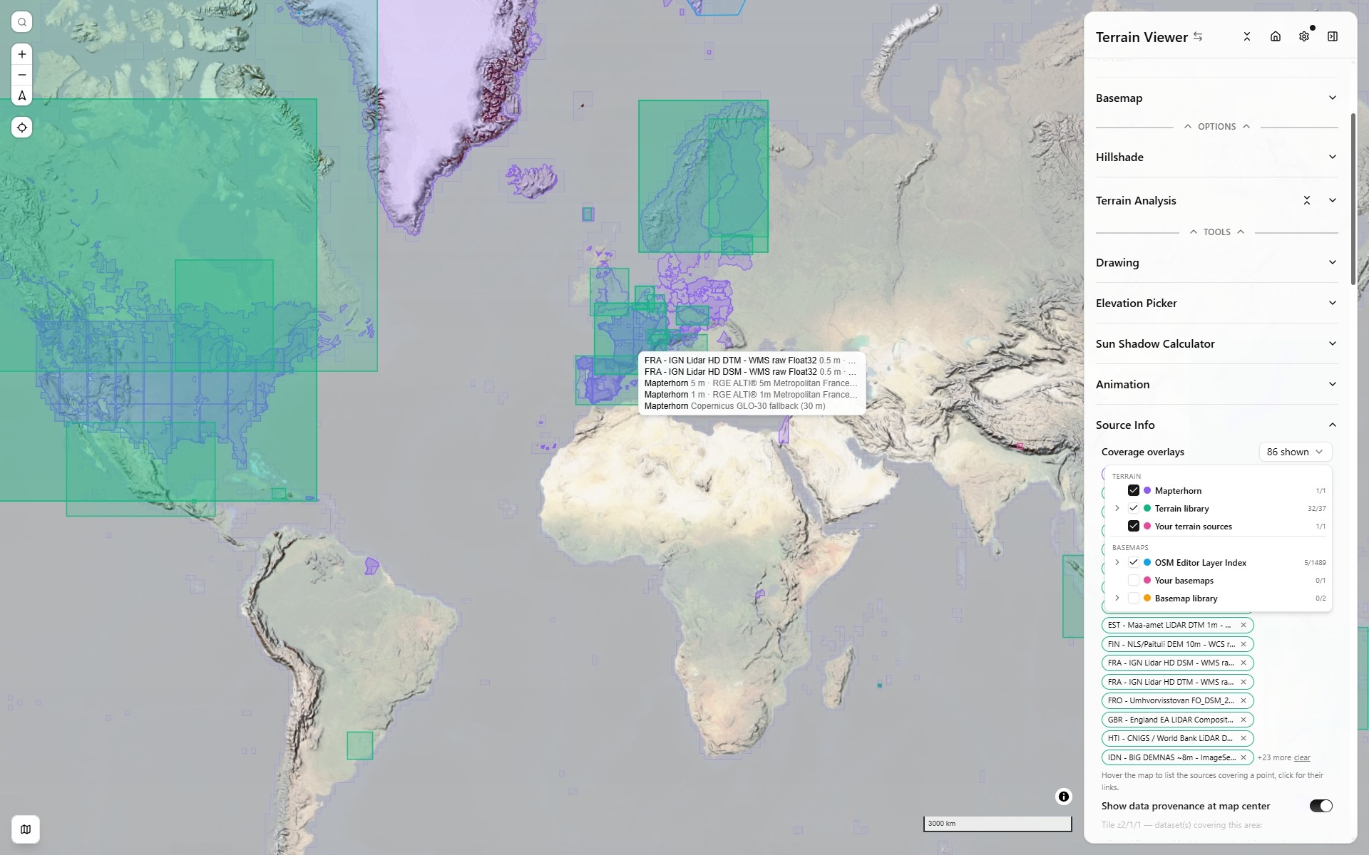
The Source Info section has a Coverage overlays picker. It draws the footprint of sources on every map view, so a blank area can be told apart from a slow one, and so you can see which national dataset or which imagery layer covers the place you are looking at before loading it.
The selection is part of the shared link (coverageOverlays), so a view you send keeps its footprints, and Source Info opens with it so the footprints have a visible origin.
A whole group is carried as its group key, not as its members: ticking the Terrain library writes ?coverageOverlays=library, not the 45 ids it stands for. Untick one entry and the other 44 spill out, because there is no longer a group to name. The foldable group keys are library and basemapLibrary — the two whose membership is fixed at build time. mapterhorn is a single footprint and always travels as itself.
The other three groups — eli, yourTerrain, yourBasemaps — name sources that only exist in your session, so a link carries their ids rather than the group key. You can still write those keys by hand: ?coverageOverlays=yourTerrain is expanded against whatever is loaded when the link opens.
What is offered
The picker is a small tree, independent of what is loaded in your Terrain and Basemap lists. Tick a group to draw all of it, or expand it (chevron on the left) and pick a handful of entries.
Terrain
-
Mapterhorn — the built-in terrain's own coverage, streamed from Mapterhorn's coverage vector tiles (
single-archive-tiles.mapterhorn.com/coverage/{z}/{x}/{y}.mvt). Each polygon carries the id of the national source Mapterhorn ingested there; areas that fall back to Copernicus GLO-30 are drawn hollow. Hovering shows the product name, producer and grid resolution, read once from Mapterhorn's attribution table. -
Terrain library — the declared bounds of every dataset in the national datasets library, loaded or not.
-
Your terrain sources — custom terrain sources you added yourself that declare bounds (Advanced section of the Add Terrain dialog) and are not library entries.
-
Bing Maps 3D (photogrammetry) — where Bing Maps 3D actually has mesh: the photogrammetry behind Bing's 3D cities and Flight Simulator. Not something this app can draw, but "is there photogrammetry here?" belongs on the same map as "is there a fine DEM here?". Includes terrain photogrammetry of parks (Rainier, Yellowstone, the Grand Canyon), not only cities.
-
Google 3D (photorealistic) — the same question for Google’s mesh. Google publishes no machine-readable coverage, and its 3D Tiles tree cannot be asked — it refines to 2 m over rural Nepal exactly as over central Paris — but the coverage layer behind its own docs page is an ordinary Maps vector layer, and that can be decoded. The layer is generalised per zoom, so three zooms are fetched and unioned; the result is simplified to about half a kilometre, which is the scale of the question. Generalising a union of tile‑clipped triangles leaves two kinds of rubbish behind — sub‑kilometre holes where triangles met imperfectly, and self‑intersections made by the simplification itself — so each merged polygon is re‑noded and its pinprick holes dropped before it ships.
-
FLAI open LiDAR — 114 open point clouds republished as COPC at hub.flai.ai. Not a DEM, but the same question: is there anything better than global 30 m here? These are real flown footprints, not bounding boxes — traced from each COPC octree’s own occupied nodes, which is why France comes out as France rather than as the rectangle around it. Click one to open it in FLAI Hub at the same view.
-
Esri Integrated Mesh — every public photogrammetric I3S scene layer on ArcGIS Online, one rectangle per service. There are about 10 900 of them and most are one drone flight over one building site, so anything under 5 km² of declared extent is dropped — a speck you cannot click is not an answer. That leaves 1 719, cities down to districts. Esri has no global photorealistic mesh — its one global 3D Buildings layer (TomTom, Vantor, Community Maps, Overture, quarterly) is modelled buildings, not imagery-derived, and declares a whole-world extent, so there is no footprint to draw and it is not one of these. None of it is renderable here, I3S being Esri’s own format, so clicking a footprint opens that one service in Esri’s Scene Viewer instead — the service alone, so nothing else in the scene collides with the mesh.
Basemaps
- OSM Editor Layer Index — the real coverage polygons of the Editor Layer Index layers whose footprint touches the current view at the moment the picker opens. Worldwide layers have no footprint and are left out.
- Your basemaps — custom basemaps with declared bounds, or added from the Editor Layer Index (those use the index polygon).
- Basemap library — the sample basemaps that declare bounds.
Reading the map
- Hover a point to list every overlay covering it in a floating box.
- Click to open the same list as a dialog, with each source's dataset page or catalog record linked.
- Selected entries show as pills under the picker. A fully selected group is one pill with its count; remove a pill to hide it, or clear to hide all.
Overlays are drawn on all views of a split or grid layout. The selection is session-only: it is not saved and not part of the share URL.
Where the footprints come from
| Group | Geometry | Source |
|---|---|---|
| Mapterhorn | Vector tiles, per national source | Mapterhorn coverage tiles + attribution.json |
| Terrain / basemap library | Bounds rectangles | bounds of each entry in lib/custom-sources.json |
| OSM Editor Layer Index | Coverage polygons | @osm-editor-kit/maplibre-editor-layer-index (bundled index, bumped weekly) |
| Your sources | Bounds rectangles | the bounds you declared in the source dialog |
| Bing Maps 3D | Merged tile rectangles, ~2.4 km | Bing's own 3D Tiles subtree availability (td1 manifest → st… subt bitstreams), crawled by docs/scripts/build-bing-3d-coverage.mjs into public/coverage/bing-3d.geojson — no API key, nothing published lists it |
| Google 3D | Decoded polygons, dissolved, ~500 m | Google’s own coverage layer, fetched from maps.googleapis.com/maps/vt at z8–z10 with a layer id minted from an API key, decoded (XOR 0x9b + protobuf + triangle mesh) by docs/scripts/google3d-coverage.ts, then unioned and simplified by docs/scripts/dissolve-google-3d-coverage.mjs into public/coverage/google-3d.geojson |
| FLAI open LiDAR | Traced octree cells, per dataset | Each survey’s COPC octree hierarchy — the overview file’s occupied nodes, read over range requests without downloading any points — by docs/scripts/build-flai-coverage.mjs into public/coverage/flai-open-lidar.geojson. FLAI’s API carries no geometry at all |
| Esri Integrated Mesh | One rectangle per scene layer | ArcGIS Online’s public search API, which returns each item’s extent, by docs/scripts/build-esri-3d-coverage.mjs into public/coverage/esri-3d.geojson — no key, no crawl. Matched on typeKeywords:"IntegratedMesh", which ArcGIS sets itself when the layer is published; the free-text tag "integrated mesh" finds 48 layers where the type keyword finds 10 900. Queried a year at a time, since search caps any one query at 10 000 items. Deduped by service URL, since the same hosted mesh is routinely registered as several items |
How the 3D and LiDAR footprints are built
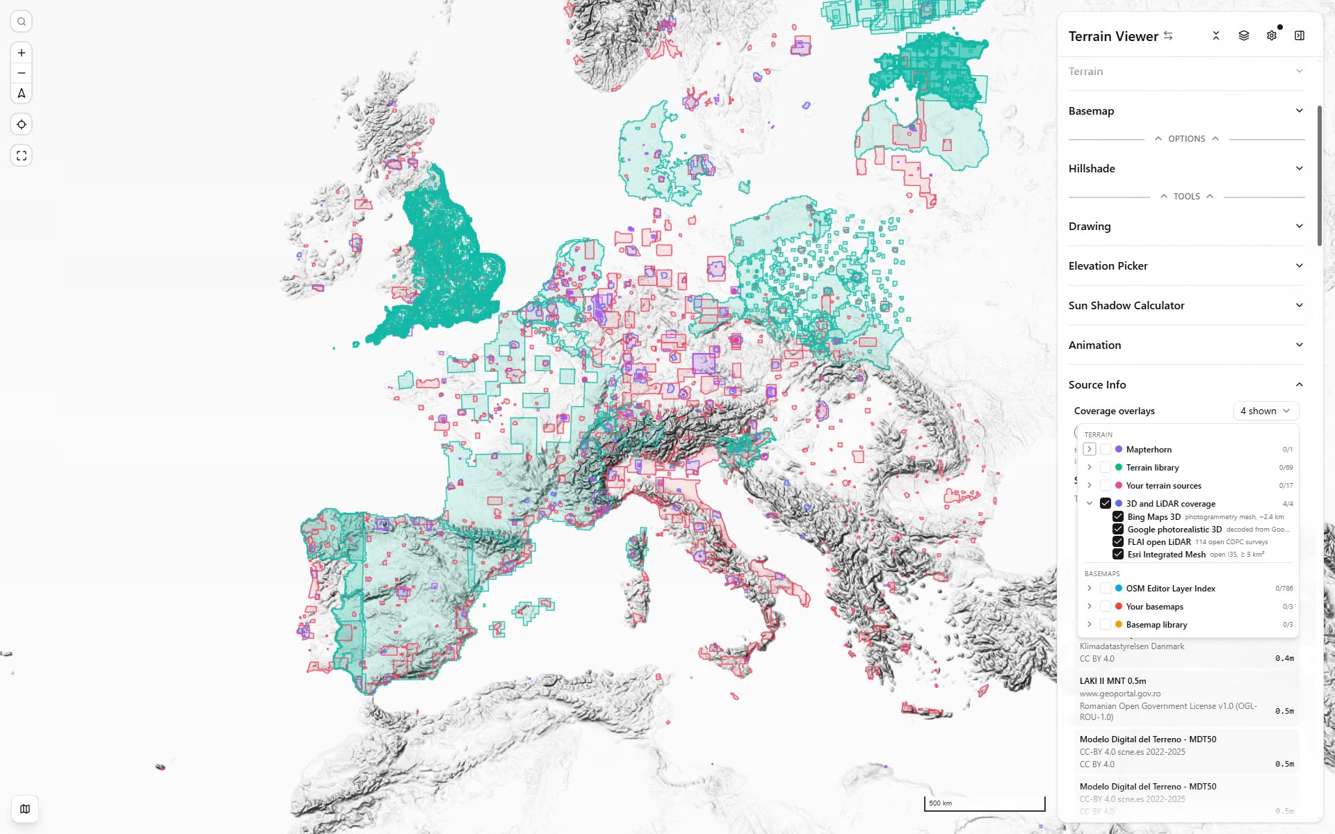
The four 3D and LiDAR overlays on one switch, over Europe - Bing (indigo), Google (rose), Esri Integrated Mesh (violet), FLAI (teal)
None of these is built by the deploy workflow. Each is a script under docs/scripts/, run by hand, whose output is committed under public/coverage/; the GitHub Action only builds the app and this docs site. Times are from one machine on 2026-09-24.
Google photorealistic 3D
Not rasterised, not screen-scraped from the Maps JavaScript API, and not derived from the 3D Tiles API — that tree refines to 2 m over rural Nepal exactly as over central Paris, so its depth says nothing about photogrammetry (measured by probe-google-3d-detail.mjs). It is Google's own coverage layer, the one drawn on the Photorealistic 3D Tiles coverage page, which turns out to be an ordinary Maps vector layer: tiles from maps.googleapis.com/maps/vt with a layer id (ml:xs:c:…) that mapConfigs:batchGet mints from a plain API key. A tile body is XOR 0x9b, then a protobuf of a pre‑triangulated mesh in tile‑local integer coordinates on an 8 192 grid.
The bug that hid behind every other fix, for the record: the decoder read each vertex delta with protobuf's zigzag rule (v/2, −(v+1)/2), and this format is not zigzag — it wants v / −(v+1). Every polygon came out deflated 2× about its first vertex, so each zoom covered exactly (½)² ≈ 25 % of central Paris, different zooms' pieces landed in different places, unions grew with every zoom added and never converged, and London and San Francisco tested "outside". That was misread, in turn, as generalisation, as a per‑tile budget and as zoom sharding. Jonathan spotted the 2× from the shape of the polygons in kepler.gl. The rule was settled by cross‑zoom agreement: with it, the central‑Paris z10 tile and its four z11 children render the same polygons (Jaccard 1.00, 96 % of the tile covered); with zigzag they were near‑disjoint (0.32, 23 %). Decoded correctly the layer is an ordinary generalised one — every zoom from z5 to z12 gives ~2.05 Mkm² worldwide and 91–96 % of that tile — so one zoom is all it takes, and the union‑of‑zooms machinery is gone.
Three stages, in this order:
- Fetch —
docs/scripts/google3d-coverage.ts fetch, one hierarchical crawl from z5 to z8: an empty tile is a fixed 36‑byte stub, so only non‑empty children are descended. 4 120 requests, 32 MB, about 10 s, into.cache/google3d/. - Decode —
google3d-coverage.ts decode --zoom 8: XOR, protobuf, triangles → rings by cancelling shared edges. Two things earlier decoders got wrong and that silently delete cities: zero‑area collinear triangles are part of the mesh and must be counted, and vertices must keep their ~0.7 % overshoot rather than be clamped to the tile box. Coordinates go from the 8 192 grid to lng/lat, so the only quantisation is the tile's own, 19 m at z8. Output.cache/google3d-z8.geojson, 17 937 polygons, about 5 s — the file to load in kepler.gl for the raw layer. The decoder was audited stage by stage on the central‑Paris tile: triangles, rings and polygons all agree to 0.3 %. - Dissolve —
docs/scripts/dissolve-google-3d-coverage.mjs: snap every ring to 3 decimals (~110 m) and clean it, drop anything under 1 000 m²; bucket by 5°×5°; union each bucket in chunks of 400, thin each partial (125 m), tree‑merge the partials pairwise until nothing merges; then per merged polygon drop holes under 1 km², simplify at ~500 m, truncate to 3 decimals, re‑node by unioning the polygon with itself, drop small holes again, drop outer rings under 1 km². 17 937 polygons → 1 601, 0.99 MB, 49 s. Outputpublic/coverage/google-3d.geojson.
Checked: central Paris 97.1 % of its tile; the wider Paris window is a single polygon of 2 894 km² with no overlaps; 20/20 on a city checklist. z9 and z10 give the same answer to within 0.2 % at the same file size — z8 is the level whose blocks read like Google Earth’s own coverage view, and it is the cheapest to crawl.
C:\Users\jonathan\.t3\worktrees\elevation-terrain-visualizer\t3code-619d1237\docs\scripts\google3d-coverage.ts
C:\Users\jonathan\.t3\worktrees\elevation-terrain-visualizer\t3code-619d1237\docs\scripts\dissolve-google-3d-coverage.mjs
C:\Users\jonathan\.t3\worktrees\elevation-terrain-visualizer\t3code-619d1237\.cache\google3d-z8.geojson       (raw decode, 17 937 polygons)
C:\Users\jonathan\.t3\worktrees\elevation-terrain-visualizer\t3code-619d1237\public\coverage\google-3d.geojson (shipped, 1.0 MB)
pnpm google-3d-fetch (needs GOOGLE_KEY) then pnpm google-3d-dissolve reproduces it in about a minute. The same endpoint and tile format also serve the layer Google Earth draws for “3D buildings where available” (ml:xsr:c:…, the id from any captured Earth bpb= request): fetch --layer-id … crawls it with no API key at all and yields blockier per‑region blobs in tiles about 4× smaller — the “which cities are covered” view rather than the parcel‑level one. Superseded but kept: build-google-3d-coverage.mjs classifies tiles by response size and needs no key (~39 km cells — the fallback if the layer id minting ever stops), build-google-3d-coverage.py is a shapely port of the decoder (delta rule fixed in step), and decode-google-3d-coverage.mjs is the earlier hand‑rolled decoder.
Bing Maps 3D
Bing serves its tf=3dv4 photogrammetry as a standard OGC 3D Tiles 1.1 implicit tileset rooted at the td1 manifest: four Web Mercator faces, each a quadtree of subt subtree binaries whose contentAvailability bitstream says exactly which tiles carry a mesh. build-bing-3d-coverage.mjs reads the 4 root subtrees, then every level‑7 subtree they mark (469), emits the content tiles at level 13 (161 276) and merges adjacent ones into rectangles. No key, 6 s. Exact by construction — it is the service's own availability data.
FLAI open LiDAR
FLAI's public API lists 114 datasets and carries no geometry. Each dataset has an overview COPC on a public bucket, and a COPC is an octree with a published index, so build-flai-coverage.mjs range‑reads the 375‑byte LAS header, the copc info VLR and the hierarchy pages, and takes the occupied nodes at level 7 as the footprint — without downloading a single point. Only nodes at or below the target level count (a COPC keeps a coarse sample at every ancestor, so counting ancestors fills the whole square). Footprints are reprojected from each dataset's CRS with proj4, definitions from epsg.io. France comes out at 33 % of its bounding box; the country is 30 %. About a minute.
Esri Integrated Mesh
ArcGIS Online's public search API, typeKeywords:"IntegratedMesh" AND access:public — the type keyword ArcGIS sets itself on publish, where the free‑text tag finds 48 layers instead of 10 887. Queried one modified year at a time to stay under the 10 000‑item cap, deduplicated by service URL, dropped under 5 km² of declared extent (drone flights over one building site), and — because access:public is the item's sharing level, not the service's — every survivor is asked for its own ?f=json anonymously and dropped if it answers with a token error or 403 (75 did). 1 644 footprints, 121 search requests plus one check per service, about two minutes.
Library bounds are the advertised extent of the service, not a survey footprint: a national LiDAR that covers 75 % of the country still shows its whole bounding box. Mapterhorn and the Editor Layer Index carry real polygons.